See your data across
space and time.
Explore linked maps, tracks, charts and tables,
with analysis calculated locally.
A desktop data-exploration project.
Explore the complete feature directory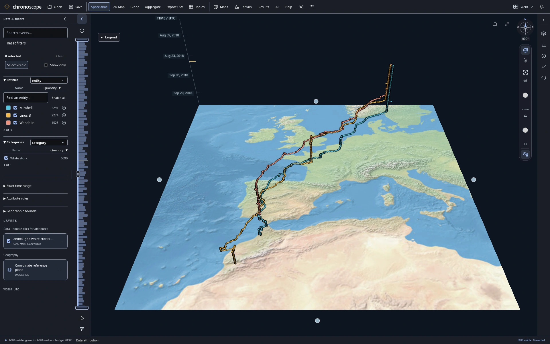
A migration drawn through time
Three white storks from Europe to North Africa; height encodes UTC time, not altitude.
17 selected views · PNG images Data & map credits ↓
A wider view.
A closer look.
Move between a 2D map, a globe and space-time views. Keep charts and source records beside the map to see the same observations from different angles.
Follow recorded journeys
One dataset. Different perspectives on movement.
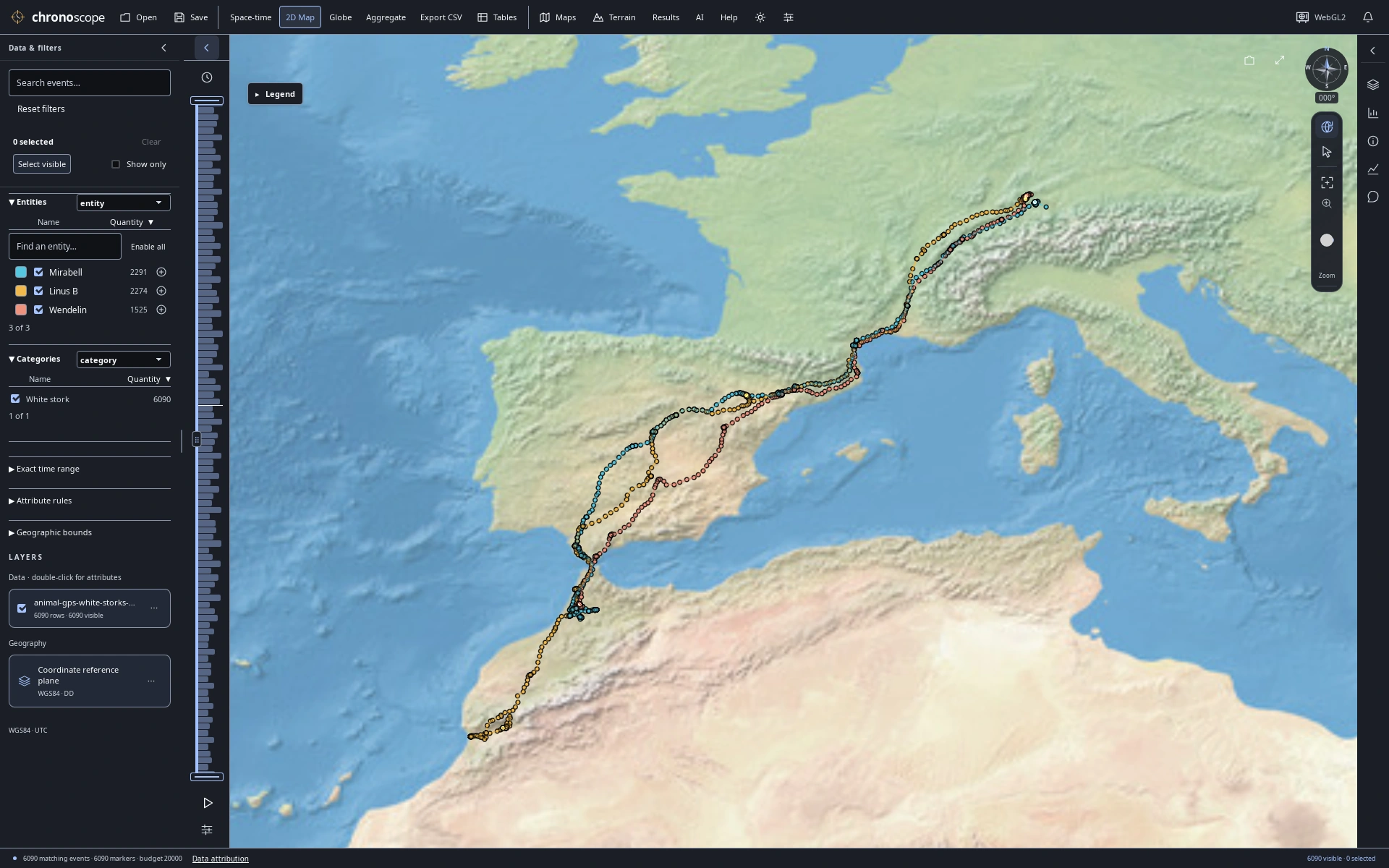
Three birds, three journeys
The same 6,090 recorded GPS fixes in a 2D map, colored by bird.
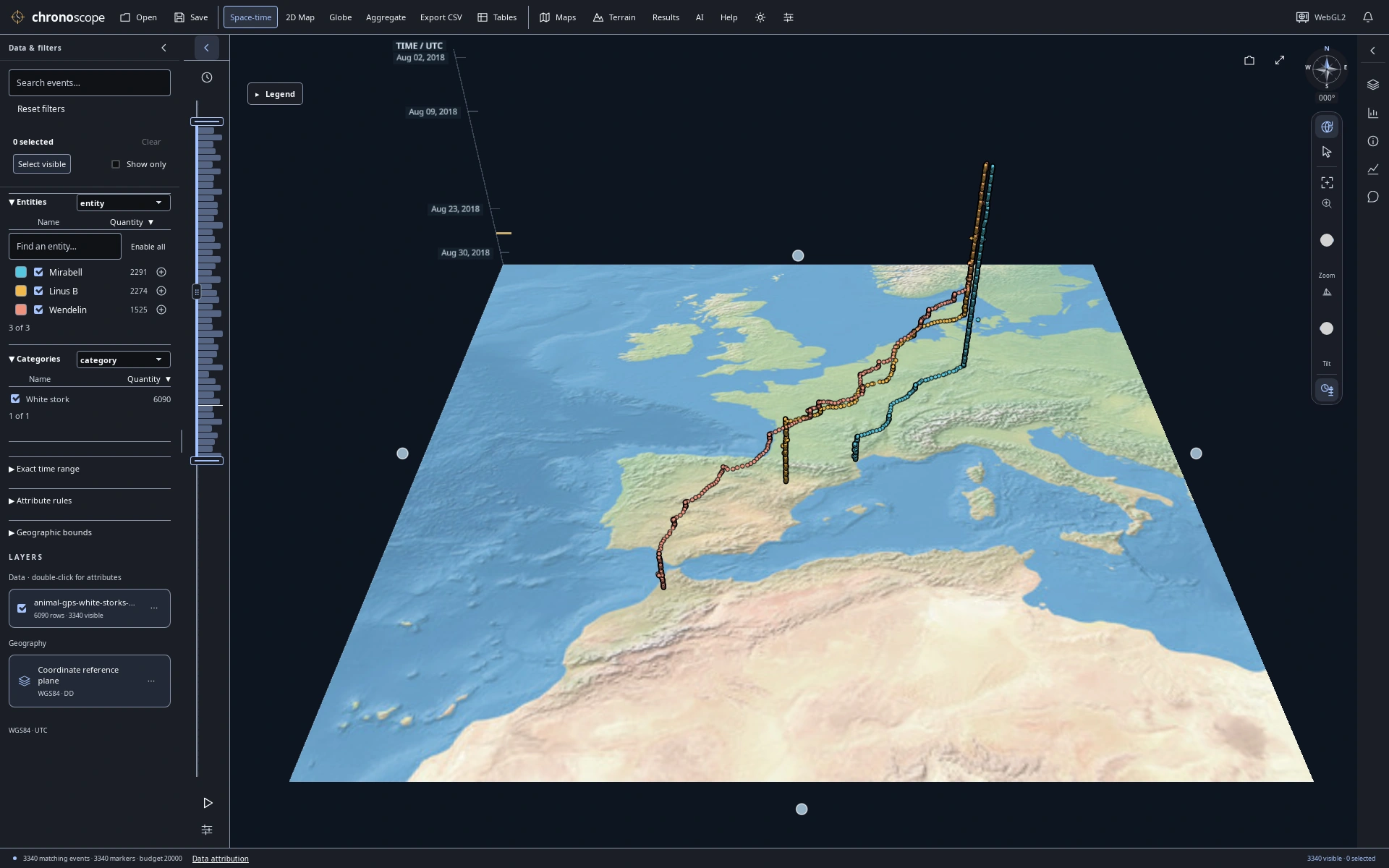
August departure
Narrow the time window to August: 3,340 matching GPS fixes from the stork dataset.
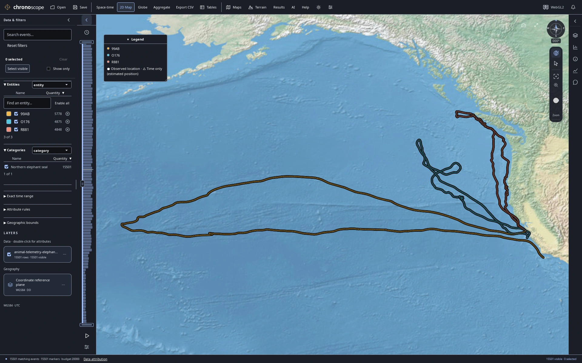
Ocean journeys
15,501 published dive summaries from three elephant seals; positions are modeled dive starts, not underwater paths.
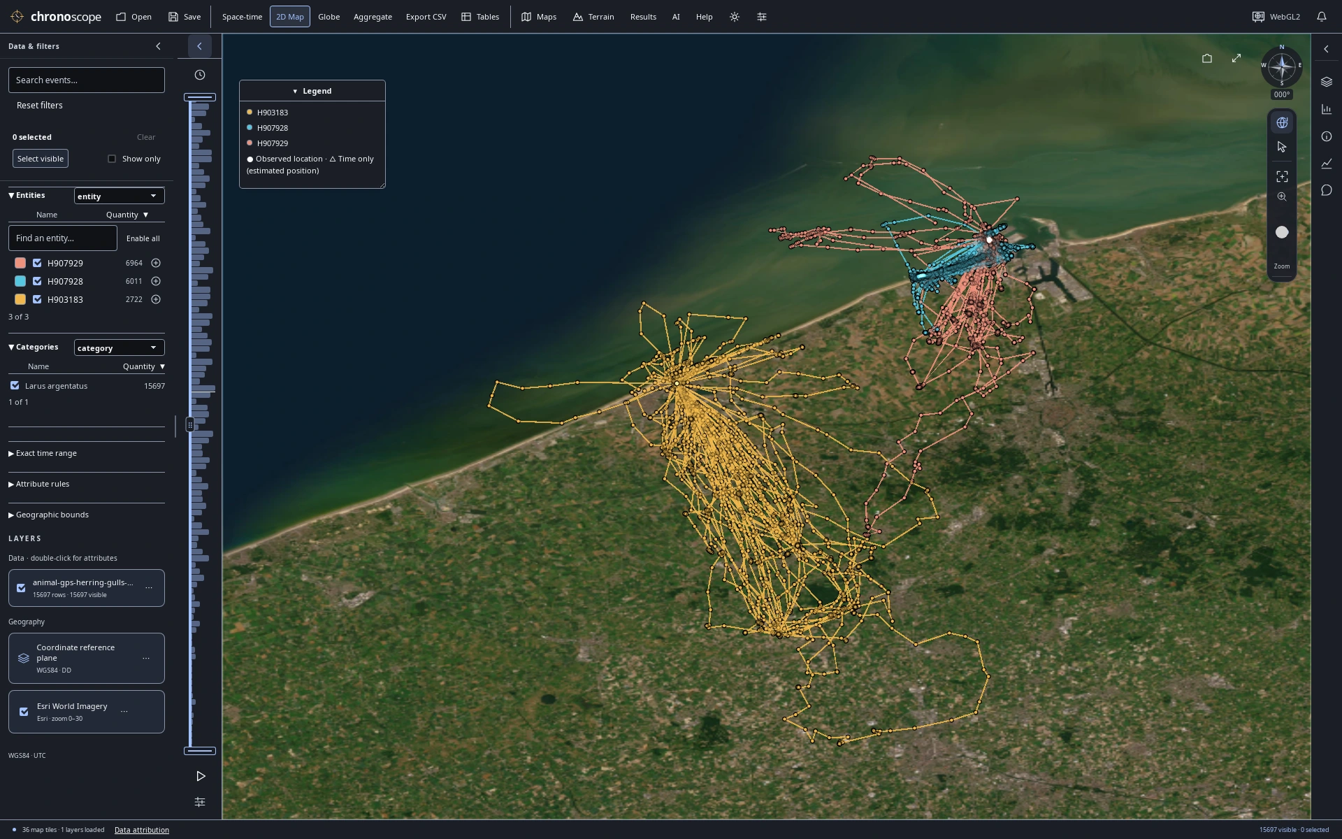
Along the Belgian coast
Three herring gulls along the Belgian coast. Connected GPS fixes do not establish continuous routes.
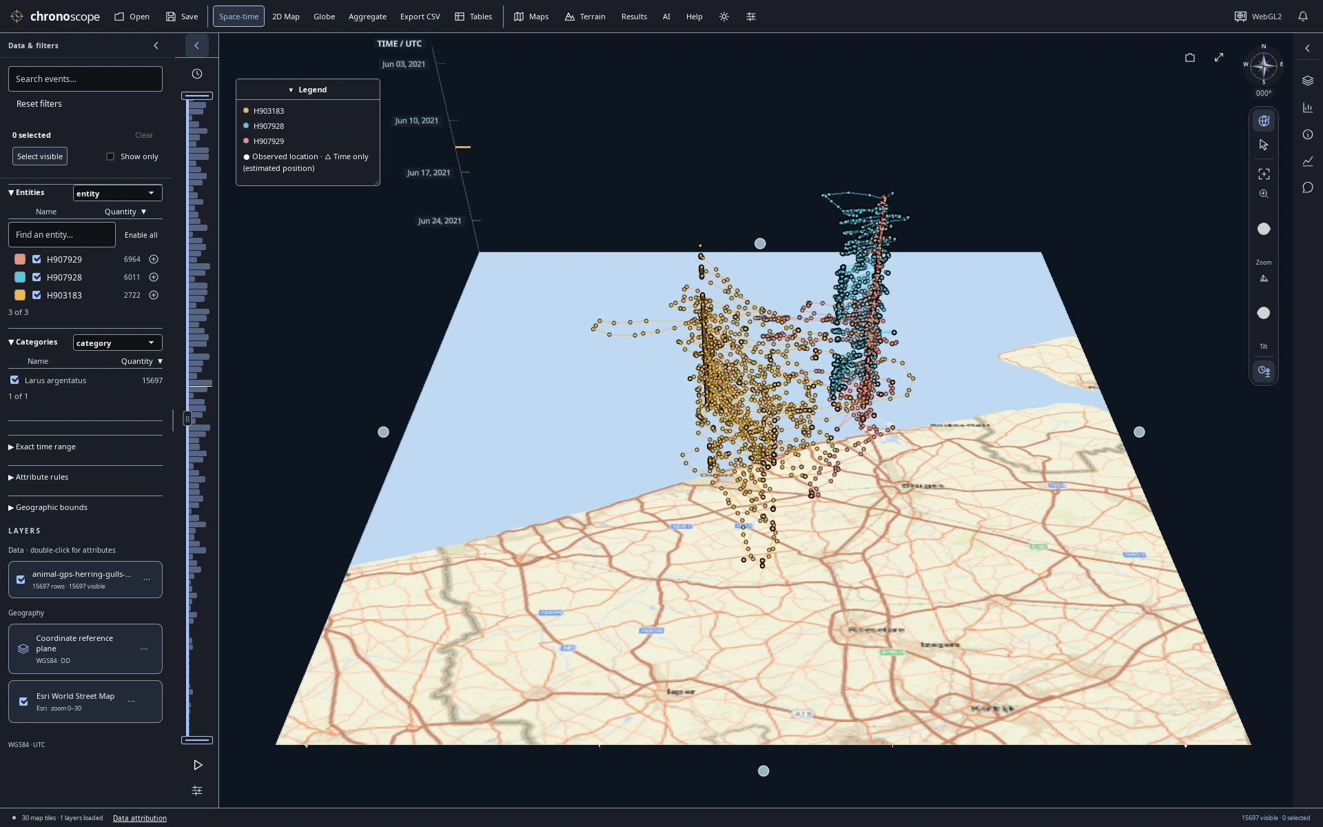
Coastal movement through June
Follow the same June 2021 gull observations through time, with UTC time on the vertical axis.
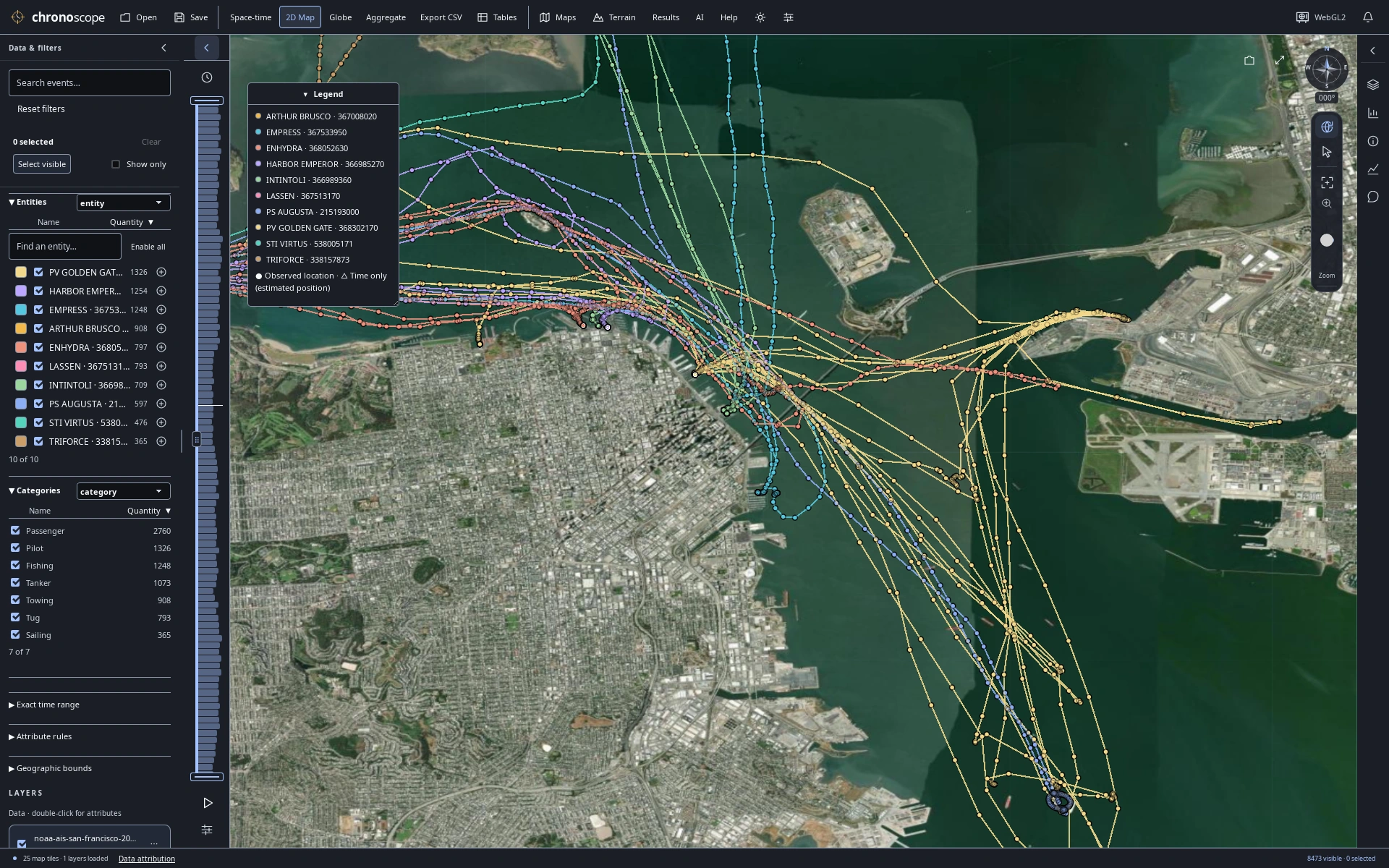
Approaching the waterfront
San Francisco Bay vessels over satellite imagery: recorded AIS samples, not independent voyages. Not for navigation.
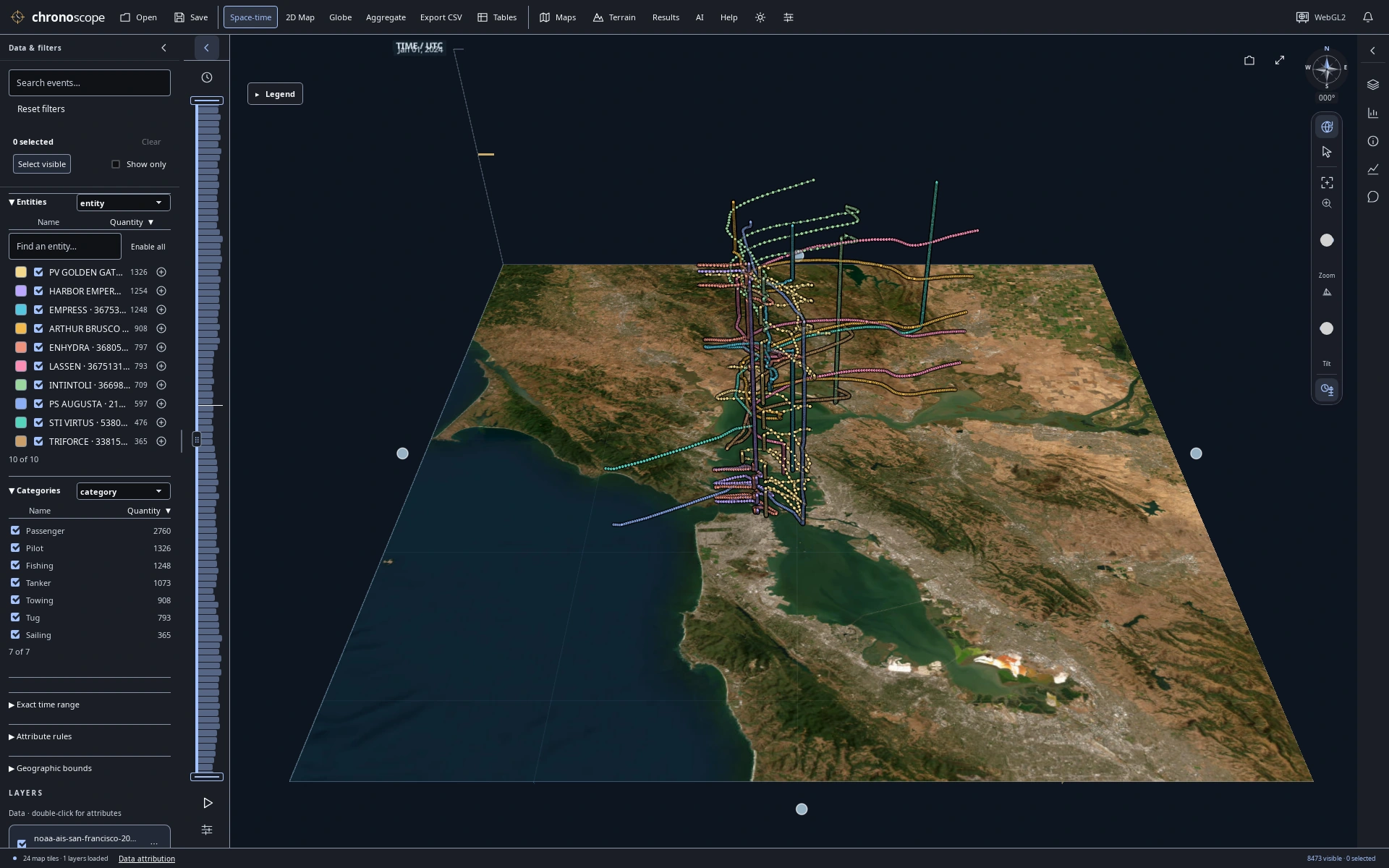
A day of traffic in three dimensions
Raise a day of Bay traffic by UTC timestamp to separate movement through time.
Compare recorded measurements
Read a chart, inspect its source records, keep the map in view.
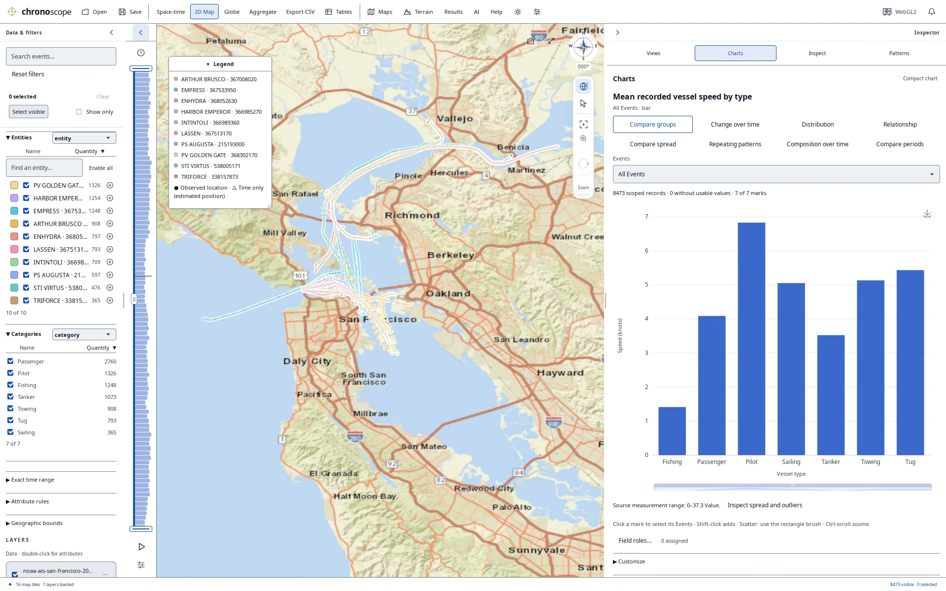
Vessel types and recorded speed
Compare recorded vessel speed by vessel type alongside the map and source records.
Explore the planet
Storm tracks and surface epicenters on a globe.
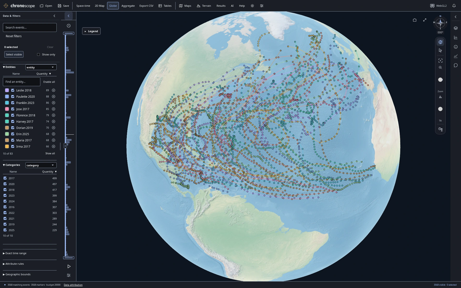
A decade across the Atlantic
3,568 NHC best-track observations connect 83 Atlantic storms from 2016–2025; reported wind is in knots.
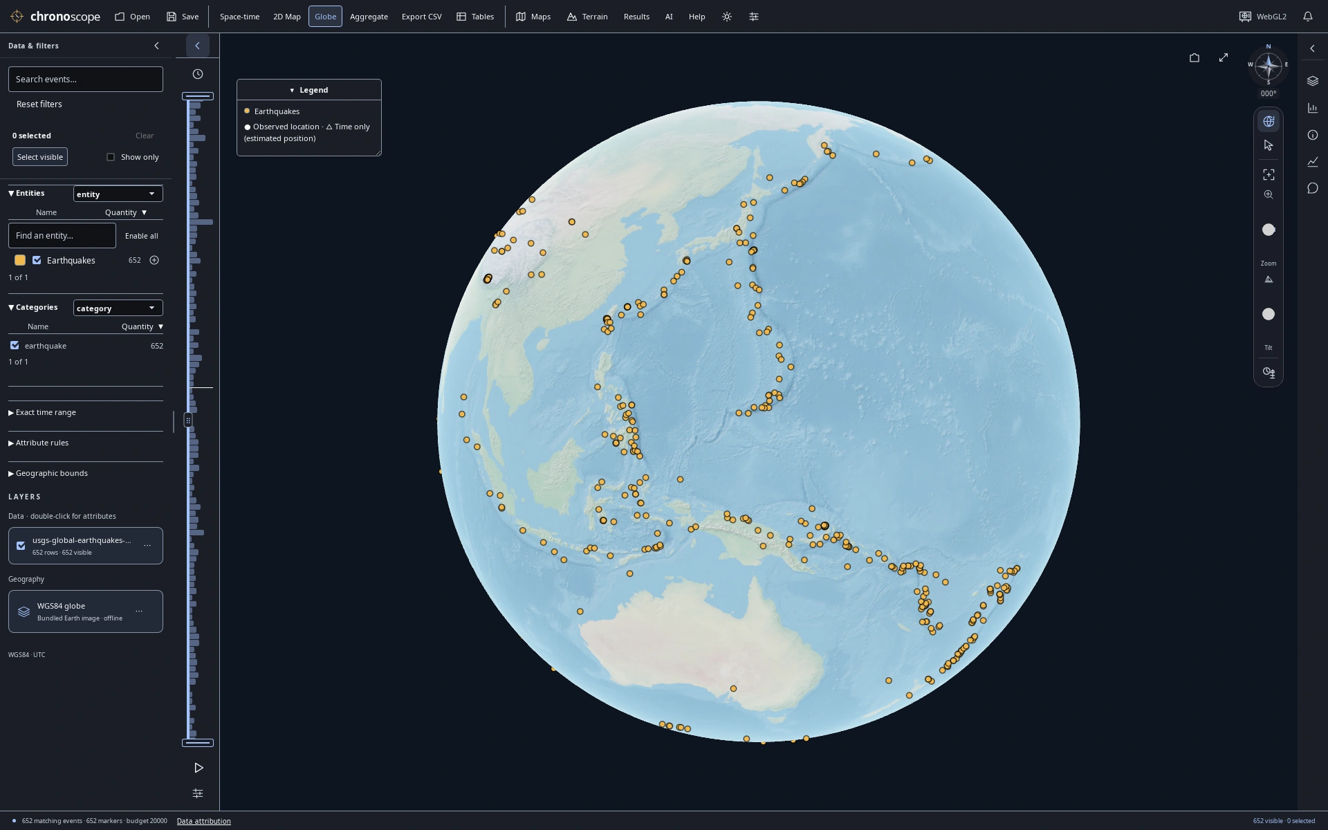
The Pacific Ring of Fire
USGS January 2025 earthquakes of reported magnitude ≥4.5. Surface epicenters, not depth; one hemisphere is visible.
Read patterns in published reports
Look closely at what counts and colors actually represent.
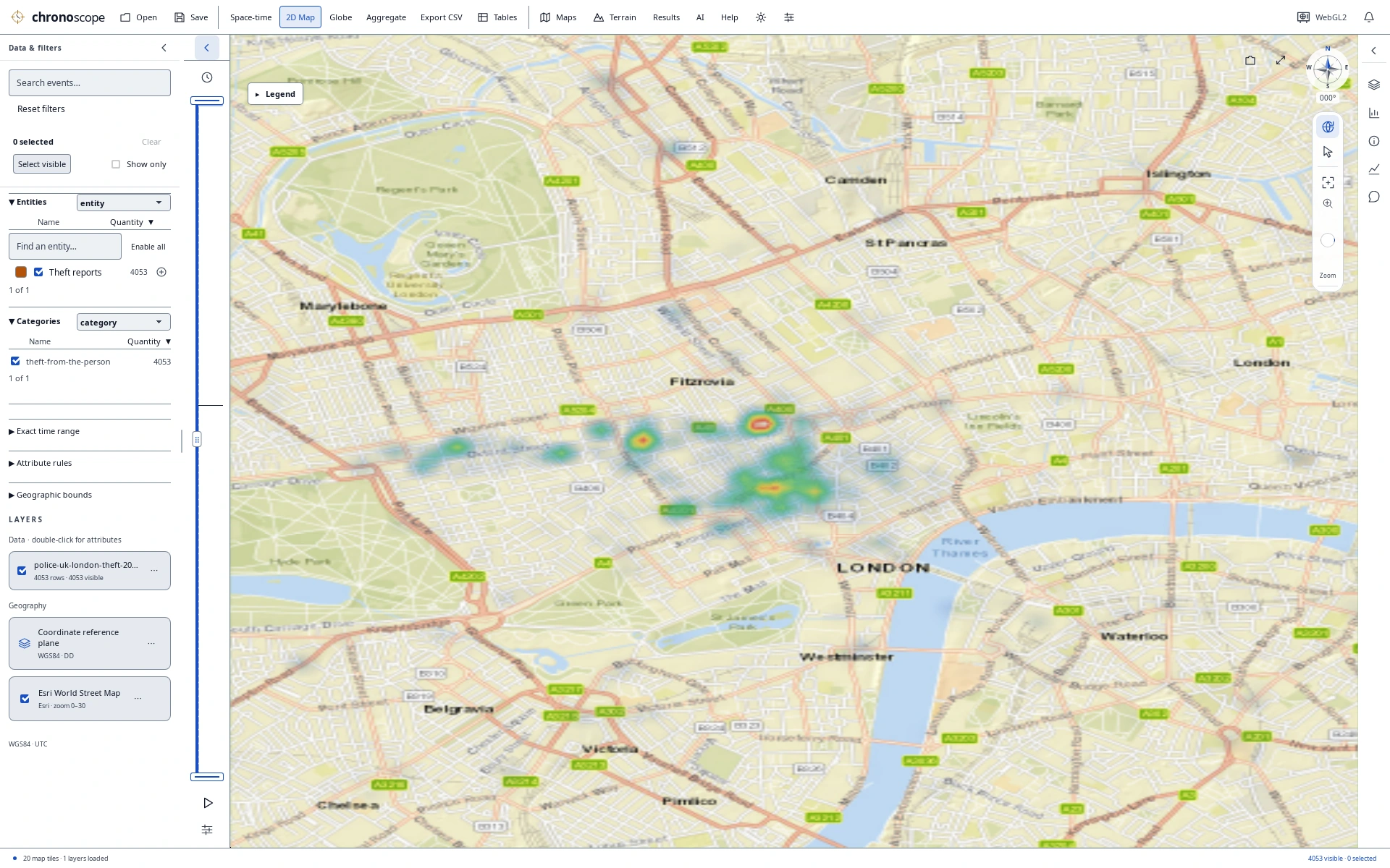
London heat map in daylight
4,053 Police.uk theft-from-the-person reports, smoothed at this zoom. Locations are approximate and dates resolve to the month—not population-adjusted risk.
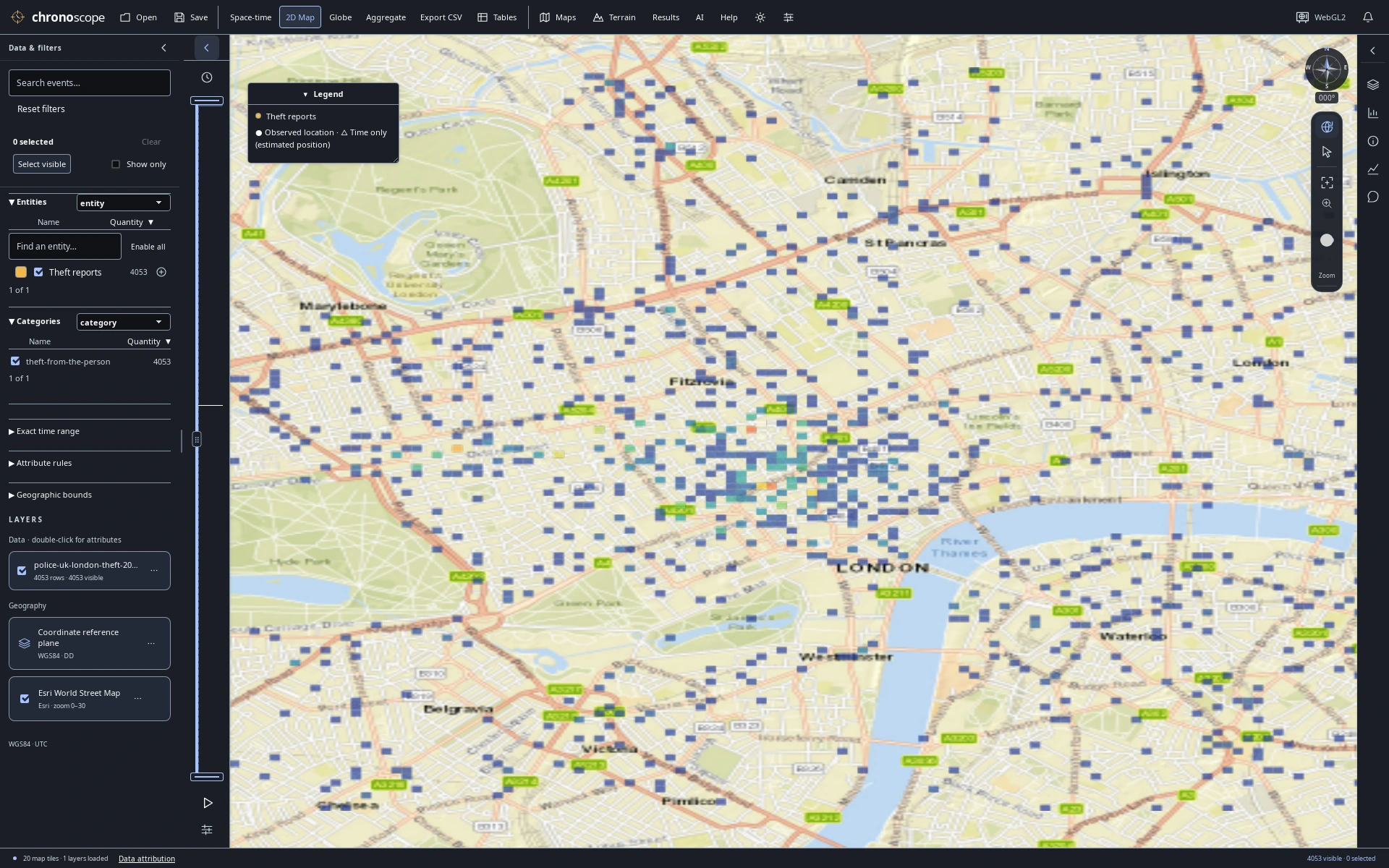
Published reports as count cells
The same published reports as display-grid counts. Cell colors summarize source records, not independent risk measurements.
Keep charts beside the map
A compact linked workspace for deeper comparisons.
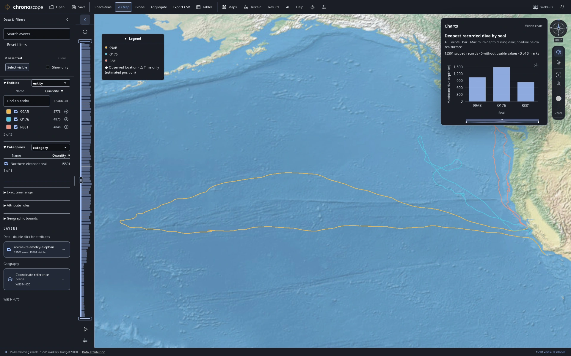
Dive depths beside ocean tracks
Keep a maximum dive-depth comparison beside the ocean tracks; depth is a recorded attribute, not map height.
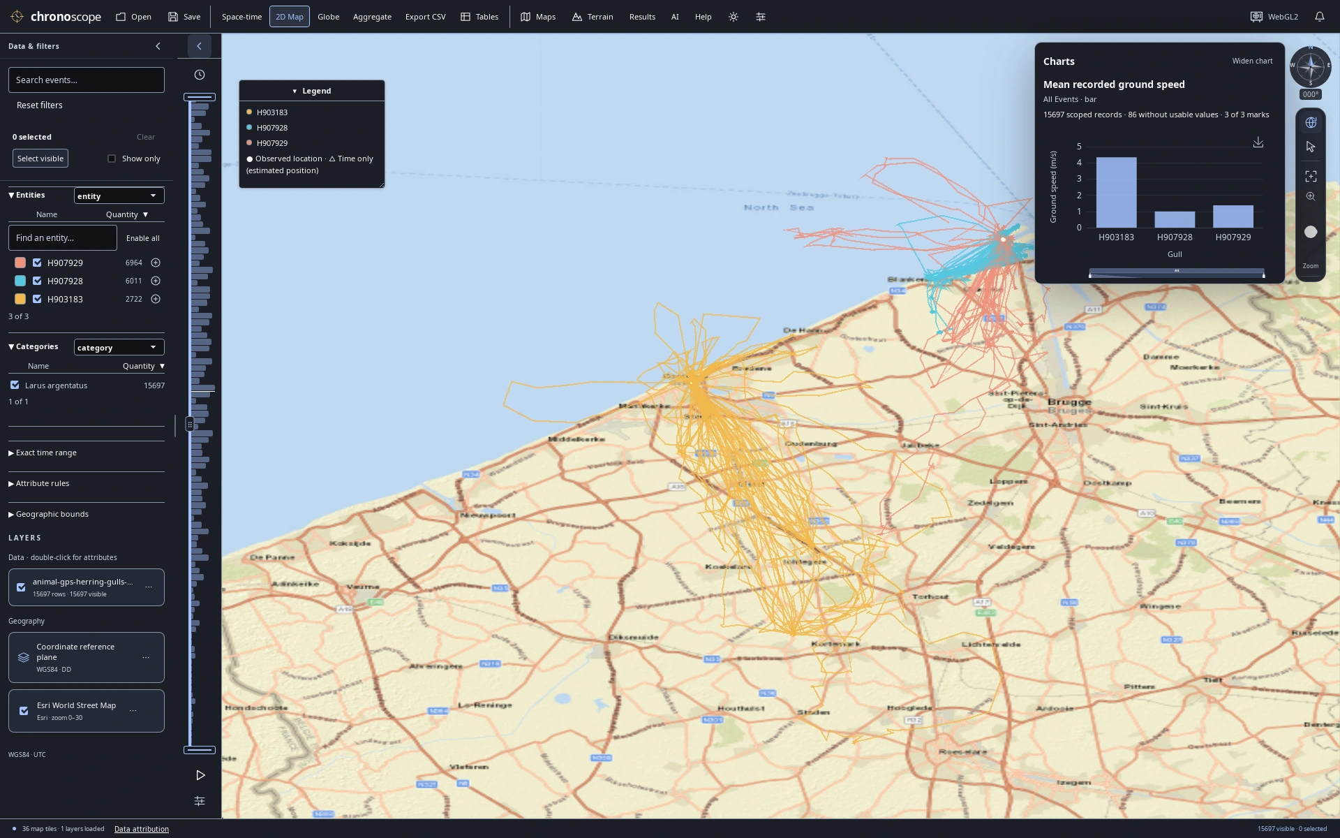
Coastal GPS with a compact speed chart
Inspect recorded gull speed alongside the coastal GPS fixes in a compact linked workspace.
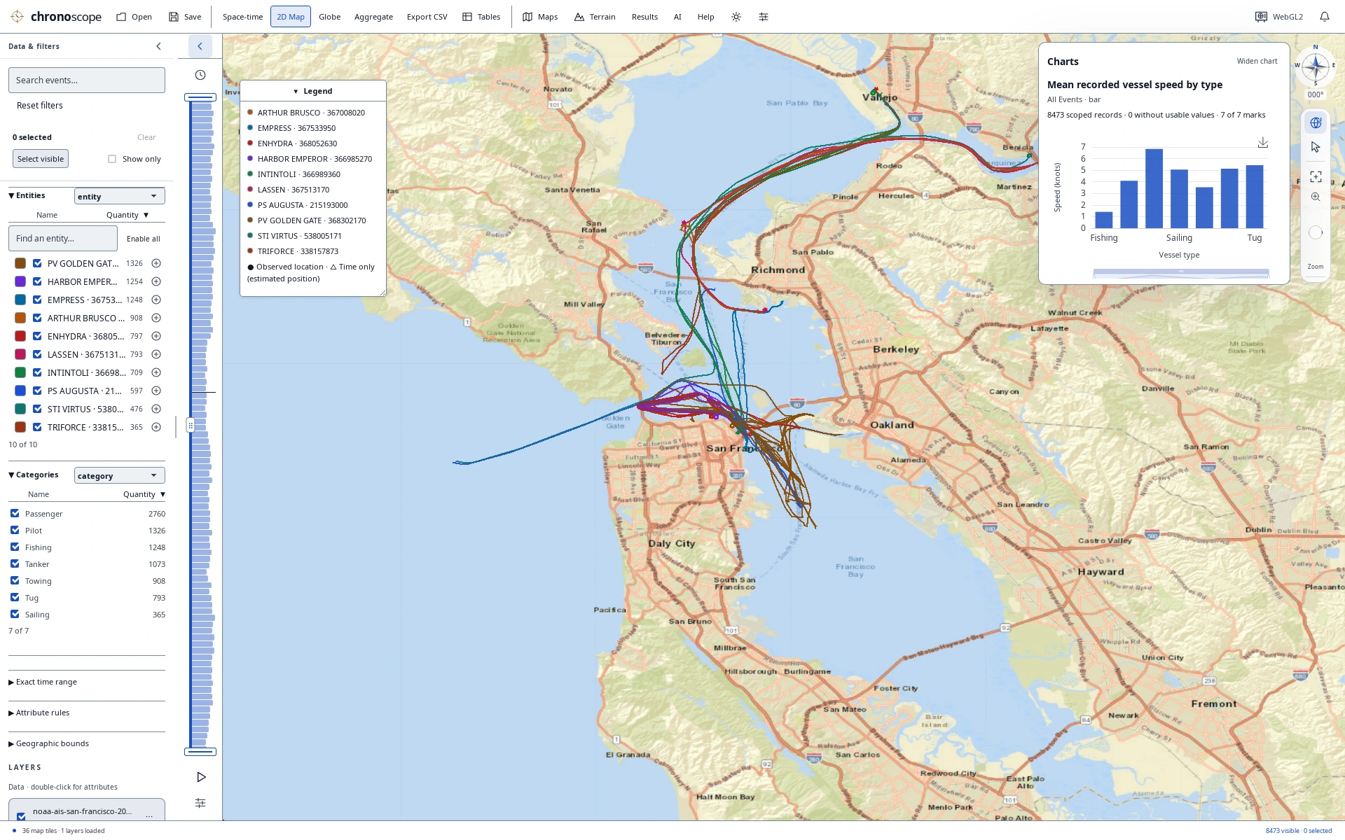
Bay traffic with a compact comparison
Compare vessel types and recorded speeds while keeping Bay traffic and the original records in view.
Terrain study
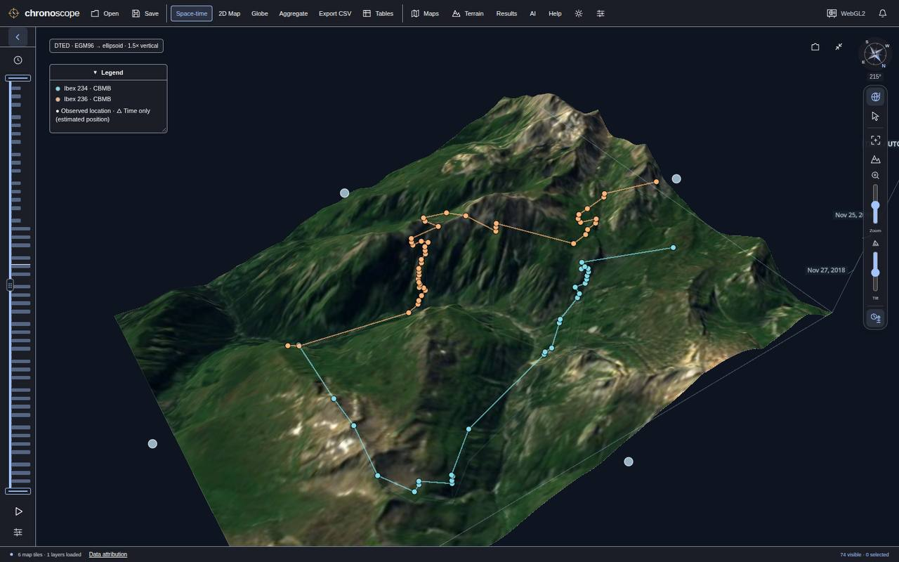
Terrain study
Animal tracks over a textured 3D terrain surface.
Bring your own
questions.
Open a bundled demo from Help → Demo datasets, or import CSV, TSV, Excel or GIS files. Filter, select, chart and save a portable .chronoscope project.
Optional SI chat and CLI/MCP tools use the same analysis engine. Online maps and connected services can send information to their providers; see the privacy guide.
Explore the source
Source version 0.15.2, unreleased. No binaries are publicly published in this clean repository yet; build from source.
View on GitHubExplore interactive AI results
Search, sort and select query results in compatible external MCP clients.
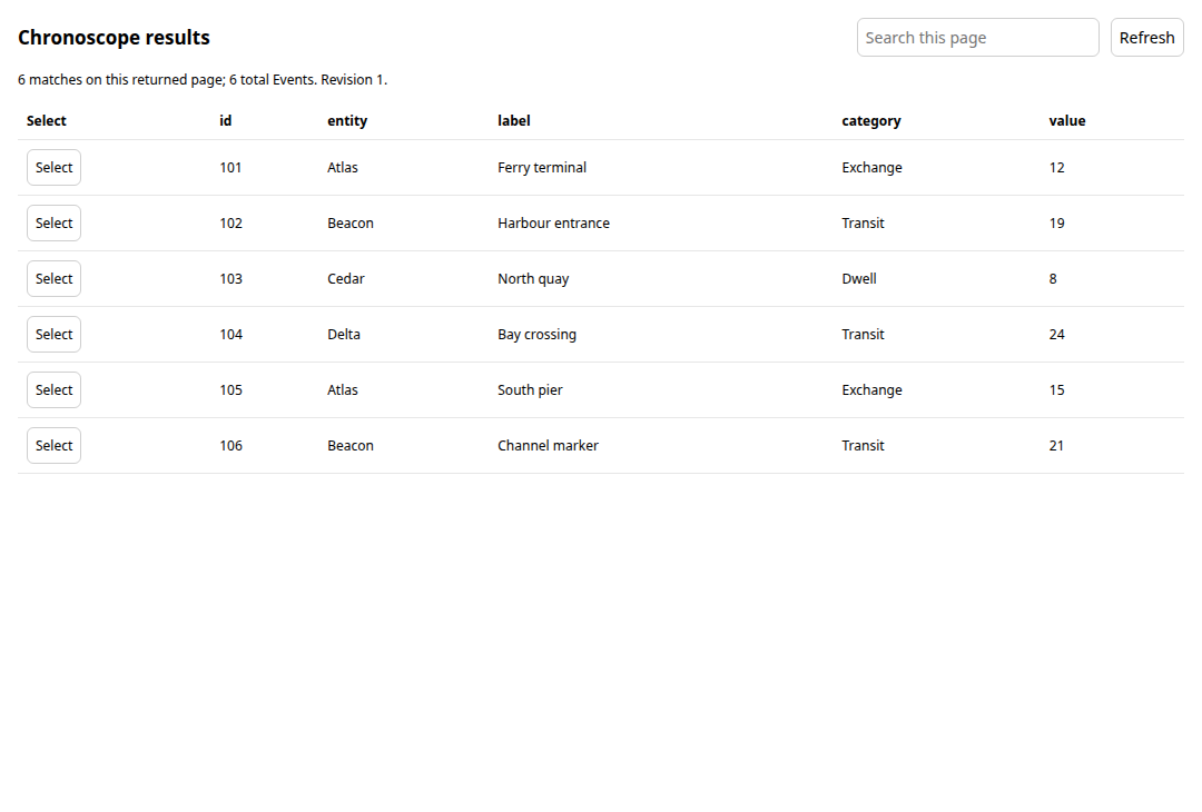
From an answer to the matching records
Search and sort the returned rows. Select a record to highlight the corresponding Events in TimeScope.
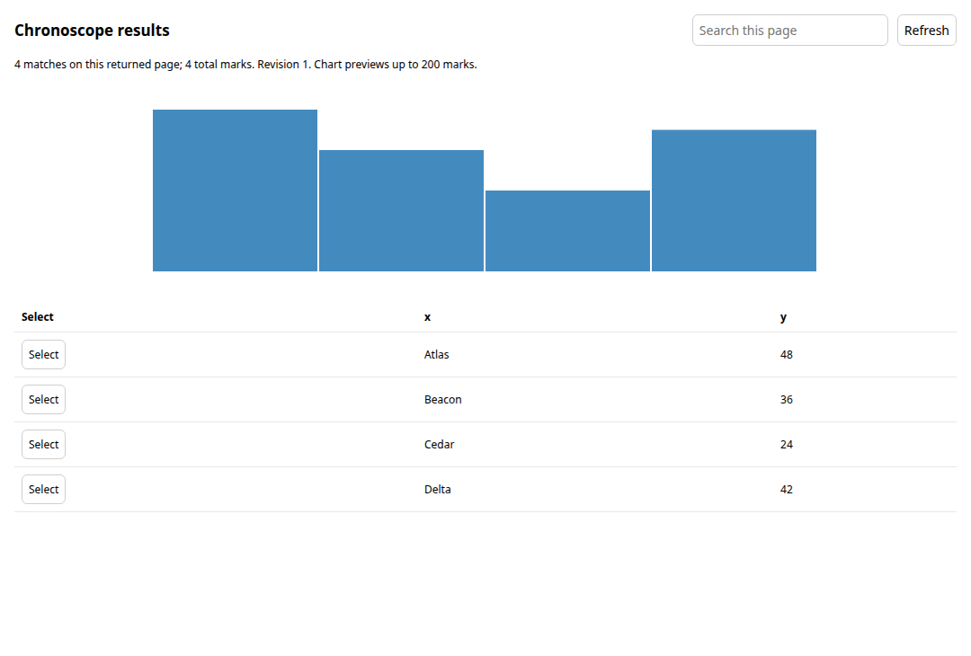
See patterns and values together
Explore a bar preview alongside its values. Select a chart mark to highlight the matching Events.
Give your tables their own space
Keep attributes beside the map, or move the table group into a separate resizable window.
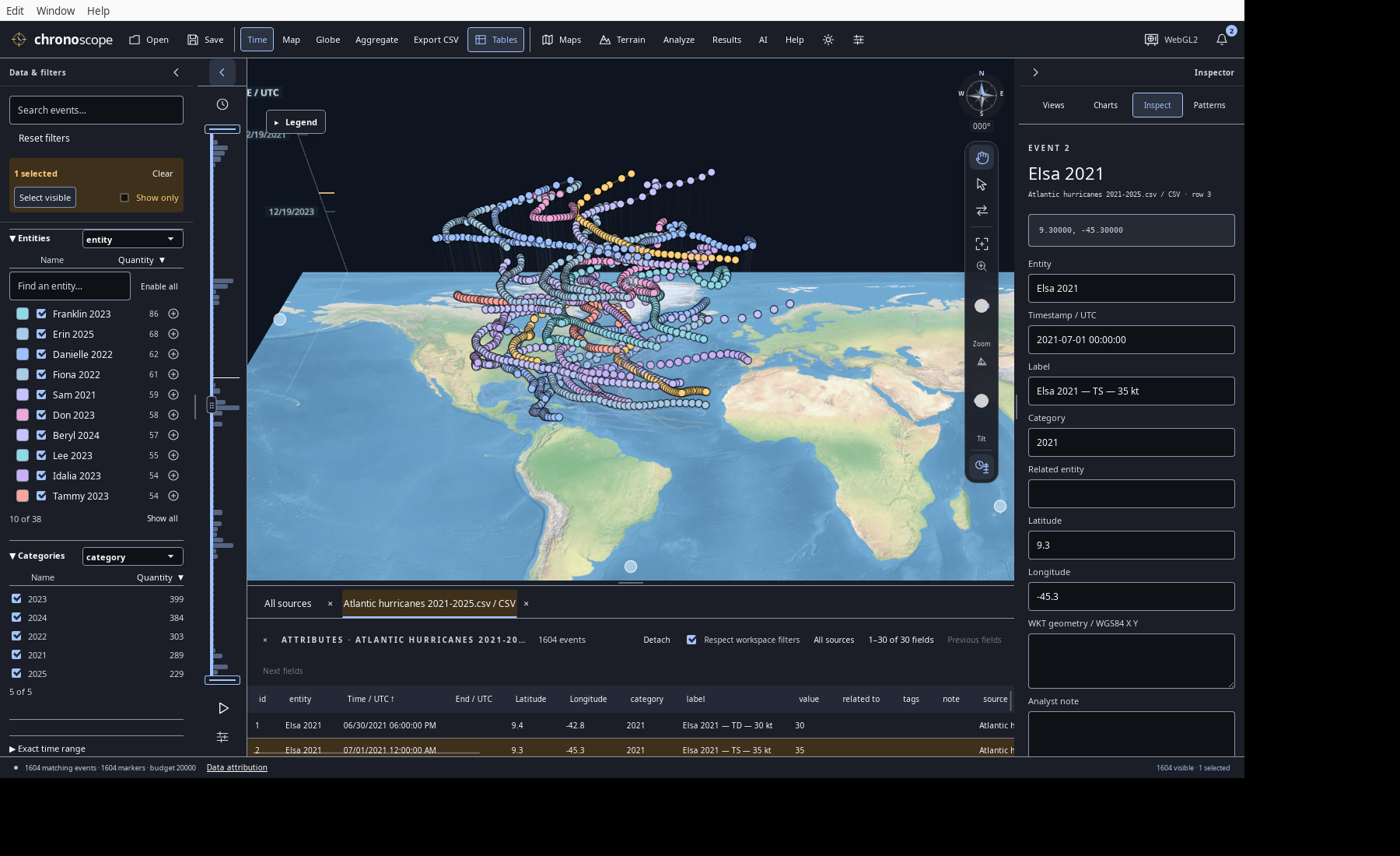
Keep the workspace in view
Open Event tables and GIS attributes in one tab group. Search original attributes, sort records and scroll through the columns.
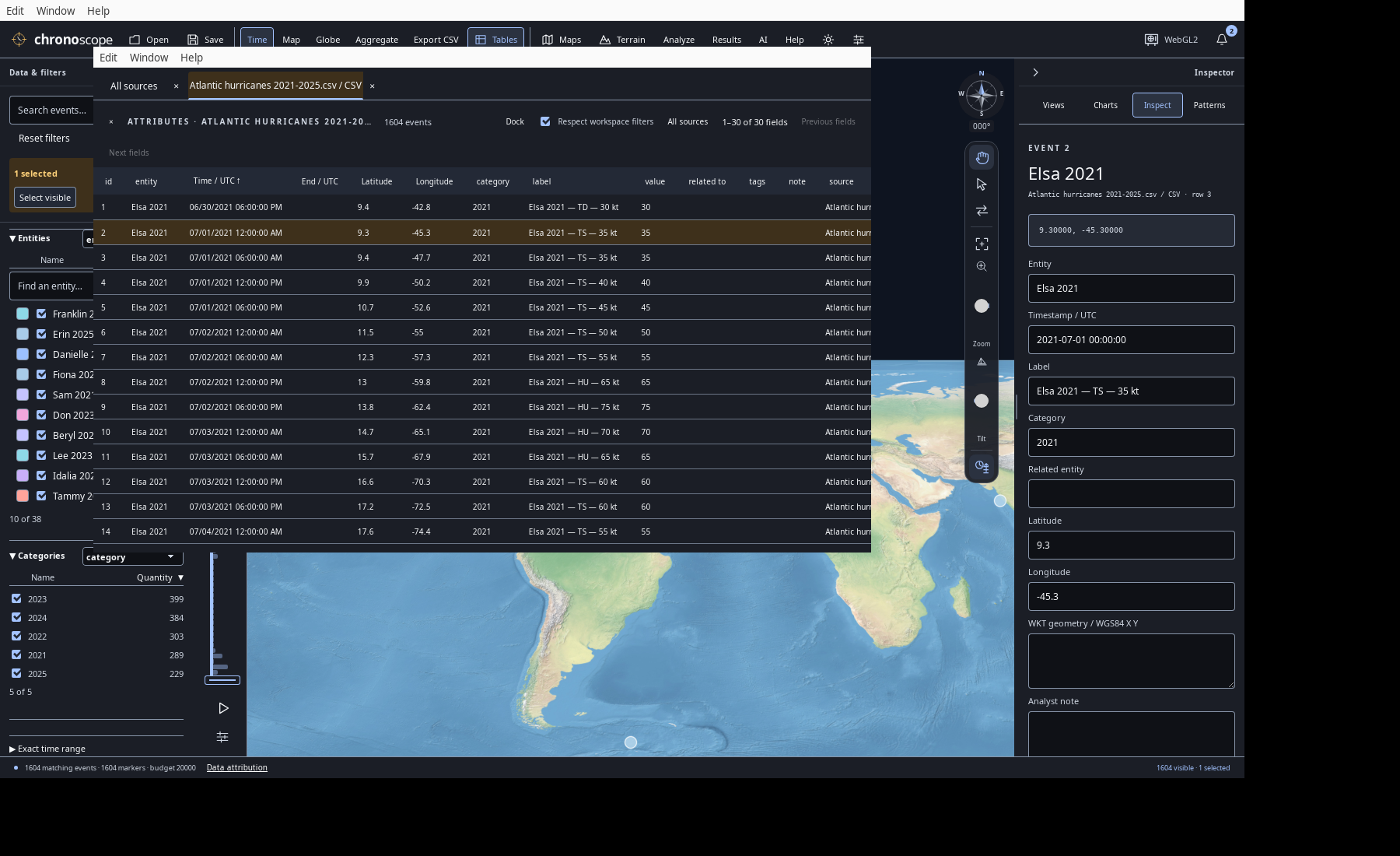
Make room to compare
Detach and resize the table group, then dock it back. Tab-specific search, sorting, scrolling and linked selection come with you.
A complete workspace.
A connected way to explore.
From the first import to a portable project, explore the tools that bring records, geography and time together.
Start with the data you have.
Bring source records into one structured workspace, with the original detail close at hand.
- Tabular files
- Open CSV, TSV, XLSX, XLS and XLSB. Choose Excel worksheets, detected delimiters and append or replace workflows.
- Guided field mapping
- Review timestamps, entities, categories, labels, values, related entities and end times in a single scrollable field grid.
- Whole-file review
- Validate every row before import, inspect missing locations and duplicate candidates, and export rejected rows with their reasons.
- Flexible date & time parsing
- Combine date and clock columns; use explicit date order, timezone assumptions, Unix units, Excel dates or custom formats. Fractional seconds stay distinct.
- WGS84 coordinates
- Import decimal degrees, UTM, polar UPS and MGRS. Preserve MGRS grid precision and keep unlocated records available for table and time analysis.
- Original detail, retained
- Keep original columns, source rows and import recipes alongside canonical fields. Use bundled demo datasets for an immediate starting point.
- Import aggregation
- Optionally summarize records during import with UTC time windows and a geographic radius while leaving the source file unchanged.
See the same records from every angle.
Move between geography and chronology without losing your filters, selections or questions.
- Three linked perspectives
- Explore a flat 2D Map, a WGS84 Globe and a Space-time view that places UTC time vertically above geography.
- Independent saved cameras
- Keep a different camera in each view. Sync the current extent and heading when you want the perspectives to align.
- Precise time windows
- Drag the time rail or histogram, move a window as a unit, enter exact UTC bounds or return to the full study range.
- Playback controls
- Play and pause through the study with millisecond-to-week increments, adjustable speed and moving-window or full-range playback.
- Tracks & time stems
- Connect successive records by entity and toggle tracks and ground stems independently. Adjust opacity, gap handling and display scale.
- Time-only records
- Keep records without coordinates in tables and time views; distinguish inferred display anchors from recorded locations.
- Value colors & legends
- Color by entity or a numeric measurement. Set the value range, title and units, and use a resizable, collapsible legend.
- Clusters, density & heat
- Explore exact-count clusters and density cells, smoothed heat maps and optional bloom. Refine by zoom and time while source records remain available.
- Globe time elevation
- Raise events by their UTC position along the globe surface normal, with independent height control and optional ground stems.
- Focused navigation
- Pan, orbit, zoom toward a location, fit your records and restore north with compass, pointer and keyboard controls.
Narrow the question. Keep the context.
A shared engine connects the map, tables, charts and results to the same working scope.
- Search & facets
- Search event text; filter by entity, category or another source field. Sort facet lists by name or quantity and switch between top entries and the full list.
- Attribute rules
- Combine text and numeric conditions with AND, including contains, equals, greater/less and missing values.
- Geographic bounds
- Apply West, South, East and North limits, including regions crossing the date line and intersection with supported event shapes.
- Linked exact selection
- Select from map marks, rows, entities, chart marks or analysis results and see the corresponding records across the workspace.
- Flexible selection gestures
- Use additive and toggle selection, keyboard ranges, box selection, Select visible and Selected events only.
- Named contexts
- Save selection groups and named views containing filters, selections, camera and display settings. Return to the same question later.
Move easily between the picture and the rows.
Inspect the source, compare attributes and make deliberate changes without leaving the workspace.
- Layer-based tables
- Open Event-layer and GIS attribute tables together in tabs. Switch between workspace-filtered rows and every record in a source.
- Search, sort & scroll
- Search original attributes, sort text or numbers and move continuously through rows and wide source columns.
- A table window of its own
- Detach the table group, resize it beside the map and dock it again with tab search, sort, scroll and linked selection intact.
- Single-record inspector
- Edit entity, UTC time, coordinates, WKT, category, label, value, related entity, tags and notes while keeping original attributes visible.
- Selection-wide changes
- Reassign, tag or delete selected records with review where appropriate. Undo and redo data edits, imports and saved contexts within the session.
- Explicit aggregation
- Preview time-and-proximity summaries, then create a summarized workspace with representative attributes, counts and mean values. Undo restores the preceding workspace.
Turn a view into a comparison.
Build linked charts from canonical or imported fields, then go directly to the records behind a mark.
- Eight guided starters
- Compare groups, change over time, distributions, relationships, spread, repeating patterns, composition over time and comparison periods.
- A full chart vocabulary
- Use bar, line, area, scatter, histogram, Tukey boxplot, UTC weekday/hour grids and paired period comparisons.
- Your fields, your scope
- Choose all, filtered or selected Events, optionally within one layer. Assign measurement, category, identifier, date/time, coordinate and unit roles.
- Flexible calculations
- Count, sum, mean, minimum or maximum; group into series, stack values, add a second Y field or choose histogram bins.
- Time at the right scale
- Use UTC buckets from milliseconds to years, unbucketed individual timestamps or explicit nonoverlapping comparison periods.
- Linked chart selection
- Click or Shift-click chart marks and brush a scatter region to select their exact source records in the map and table.
- Spread & association
- Inspect quartiles, whiskers and outliers; add a full-scope ordinary least squares trendline to a scatter chart.
- Presentation & presets
- Edit titles, labels and known units; resize the chart pane or use a compact map card. Save named chart presets with the workspace.
Go deeper, without handing off your data.
Run structured analysis locally in Rust, from guided checks to more specialized methods.
- Four guided analyses
- Profile data, find duplicate groups, detect numeric outliers with IQR or z-score thresholds, and summarize trajectories—without an AI model or API key.
- Statistical pattern scan
- Screen chosen numeric measurements for outliers, field and time associations, unusually long gaps and repeating event-count timing.
- Spatial & movement tools
- Explore proximity, stationary periods, speed thresholds, gaps and space-time clusters with adjustable distance, duration and time tolerances.
- Recorded-trajectory summaries
- Calculate WGS84 geodesic statistics between recorded samples, with missing locations and same-time conflicts made explicit.
- Reusable results
- Keep completed analyses with their methods, parameters, scope and exclusions. Select associated records; changed source data marks older results stale.
- Progress & cancellation
- Run long analyses as background jobs with progress and Cancel, while the original source records remain unchanged.
- 19 engine capabilities
- Access profiles, grouping, duplicates, quantiles, histograms, outliers, correlation, comparisons and time series through the engine, CLI or SI.
- Specialist methods
- The same catalog includes one-sample and Welch t-tests, chi-square, regression, k-means, PCA, periodicity, graph analysis, trajectories and similar-text ranking.
Bring the surrounding geography with you.
Combine timestamped Events with reference layers, imagery and elevation in the established TimeScope workspace.
- Vector & geographic files
- Open GeoJSON, TopoJSON, Shapefile, vector GeoPackage, KML/KMZ, CZML and GPX as supported reference layers or import their timestamped data as Events.
- Lines, areas & collections
- Import WGS84 WKT points, lines, polygons with holes, multipart geometries and collections. Preserve original geometry text and full shapes.
- Polygon anchors
- Use explicitly derived surface-centroid markers and tracks for polygon Events, while retaining the boundary geometry. Toggle anchors independently.
- 3D reference content
- Add local 3D Tiles and glTF/GLB reference models with explicit WGS84 placement, height and scale.
- Reference-layer controls
- Name, show, hide, fit and remove GIS layers, inspect their attributes and convert supported layer sources into Events.
- Streets & custom imagery
- Use the built-in Streets basemap or connect custom WMTS servers. Choose layer, matrix, style, date and resolution.
- A composable map stack
- Combine sources with independent opacity, drawing order and zoom visibility rules; save the stack with your workspace.
- Offline map resources
- Use the bundled Natural Earth reference and a private disk tile cache. Cache-only mode lets you revisit downloaded map resources offline.
- Terrain context
- Use bundled world elevation or load DTED Levels 0, 1 and 2. Fit coverage, adjust display exaggeration and drape supported imagery over terrain.
- Explicit vertical datums
- Choose EGM96 mean-sea-level or WGS84 ellipsoidal heights for terrain display, keeping source elevations intact.
- Protected map services
- Connect supported client-certificate WMTS services through platform authentication, with local identity choices and visible map credits.
Connect assistance to the real workspace.
Use optional AI and automation through the same validated operations that power the application.
- Choose an SI service
- Connect an OpenAI-compatible model with tool support, including a compatible local service. Filtering, selection, views and analysis use the shared Rust engine.
- Rich, flexible chat
- Read formatted responses, math, tables, charts, sources and map attachments. Keep chat docked or detach it into a separate window.
- Permissions you control
- Allow record changes per request, grant a scoped folder for file operations and revoke access. Connection credentials stay out of portable projects.
- Focused AI actions
- Request explanations of completed results or review editable tag suggestions before applying them. Choose available Apple-local or connected-service generation explicitly.
- Connect external MCP tools
- Discover tools from remote MCP services or trusted local executables. Grant query or action access individually, with separate per-message permission for external actions.
- Repeatable CLI workflows
- Import, query, analyze, edit and save through the same engine using command-line or JSON operations.
- MCP workspace access
- Expose scoped projects through stdio MCP, or enable agent access to work with the live desktop session and its current selection and views.
- Interactive MCP results
- In compatible clients, search and sort query results or explore a chart preview, then select matching records back in TimeScope.
- Capture & recording
- Capture the map, main app or detached SI window through desktop tools. On supported macOS builds, record a native window as MP4 with an available FFmpeg encoder.
Keep the work, not just a screenshot.
Carry your records and working context forward, with local recovery and a workspace that fits the way you explore.
- Portable .chronoscope files
- Save records, original attributes, linked local GIS assets and loaded terrain in one portable workspace. Open it without the original source folders.
- Your working context, restored
- Retain filters, selections, groups, cameras, named views, chart presets, map layers, tables, layout, coordinate settings and import recipes.
- Save, copy & compatible reopen
- Save to the current file, create a separate copy and reopen supported legacy Chronoscope formats. Atomic replacement protects the previous file until a save completes.
- Automatic local recovery
- Keep automatic session copies and recover previous-session checkpoints through Notifications. Explicitly saved source documents are not overwritten by autosave.
- Useful CSV extracts
- Export visible selected records, or all visible rows when nothing is selected, with original attributes and source information. Spreadsheet-formula text is escaped.
- A workspace that adapts
- Resize and collapse side panes, use floating pane rails, detach tables and chat, and switch charts between compact and wide layouts.
- Personal display preferences
- Choose system, light or dark appearance; DD, UTM or MGRS coordinates; date and clock formats; and the display marker budget.
- Keyboard-first controls
- Use familiar open/save/undo shortcuts, table navigation, accessible pane splitters, focus-managed dialogs and map navigation keys.
- Help close at hand
- Open the built-in user guide and shortcuts, try offline demo datasets, revisit recent workspaces and inspect local diagnostic outcomes.
Bring your own questions.
Keep every perspective connected.
Behind the views
Open any image for its full resolution.
Data sources, interpretation & map credits
Data sources and interpretation
Storks — pictures 1, 4, 6
6,090 GPS fixes · 3 white storks · July–September 2018.
Three white storks, Europe to North Africa. Vertical height encodes UTC time; the lines connect recorded GPS fixes.
Seals — pictures 12, 54
15,501 dive summaries · 3 northern elephant seals · 2004.
15,501 published dive summaries from three northern elephant seals. Map positions are modeled dive-start locations; depth remains an attribute.
Gulls — pictures 17, 20, 56
15,697 GPS observations · 3 herring gulls · June 2021.
15,697 June 2021 GPS observations of three herring gulls. Stienen et al. / INBO / LifeWatch, CC0. Connected fixes do not establish continuous routes.
**Data:** Stienen et al. (2022). HG_OOSTENDE v4. INBO / LifeWatch / VLIZ. CC0 1.0. doi:10.5281/zenodo.6594838..
Vessels — pictures 23, 24, 27, 57
8,473 AIS observations · 10 vessels · San Francisco Bay, 2024.
8,473 AIS observations, 1 January 2024. NOAA / USCG / BOEM / MarineCadastre. Colors distinguish vessels. Recorded samples, not independent voyages; not for navigation.
Hurricanes — picture 28
3,568 source observations · 83 Atlantic storms · 2016–2025.
3,568 original NHC best-track observations for 83 storms, 2016–2025. Colors help separate storm tracks. Tracks connect reported fixes; maximum sustained wind is in knots.
Earthquakes — picture 35
652 source events · Reported magnitude ≥4.5 · January 2025.
652 USGS-authored earthquakes of reported magnitude ≥4.5, January 2025. Surface epicenters; depth is an attribute. One globe view shows one hemisphere.
Crime — pictures 41, 42
4,053 published reports · Approximate locations · January 2025.
4,053 Police.uk theft-from-the-person reports, January 2025. Locations are anonymized approximations; dates resolve to the month. Picture 41 shows smoothed source-record counts; picture 42 shows counts in display-grid cells at this zoom. These are not population-adjusted risk scores. OGL v3.0.
Map credits
- Pictures 1, 4, 6, 12, 28, 35, 54: Natural Earth II shaded relief and water · public-domain reference artwork.
- Pictures 17, 23, 24: Esri World Imagery · Source: Esri, Vantor, Earthstar Geographics, and the GIS User Community.
- Pictures 20, 27, 41, 42, 56, 57: Esri World Street Map · Sources: Esri, HERE, Garmin, USGS, Intermap, INCREMENT P, NRCan, Esri Japan, METI, Esri China (Hong Kong), Esri Korea, Esri (Thailand), NGCC, (c) OpenStreetMap contributors, and the GIS User Community.
Map credits above are preserved from the capture catalog. Data and map content retain their respective terms; inclusion here is not blanket third-party license clearance. See repository third-party notices, bundled demo sources, and the linked source providers. The Police.uk material contains public sector information licensed under the Open Government Licence v3.0.